A tutorial on Differential Evolution with Python
I have to admit that I’m a great fan of the Differential Evolution (DE) algorithm. This algorithm, invented by R. Storn and K. Price in 1997, is a very powerful algorithm for black-box optimization (also called derivative-free optimization). Black-box optimization is about finding the minimum of a function \(f(x): \mathbb{R}^n \rightarrow \mathbb{R}\), where we don’t know its analytical form, and therefore no derivatives can be computed to minimize it (or are hard to approximate). The figure below shows how the DE algorithm approximates the minimum of a function in succesive steps:
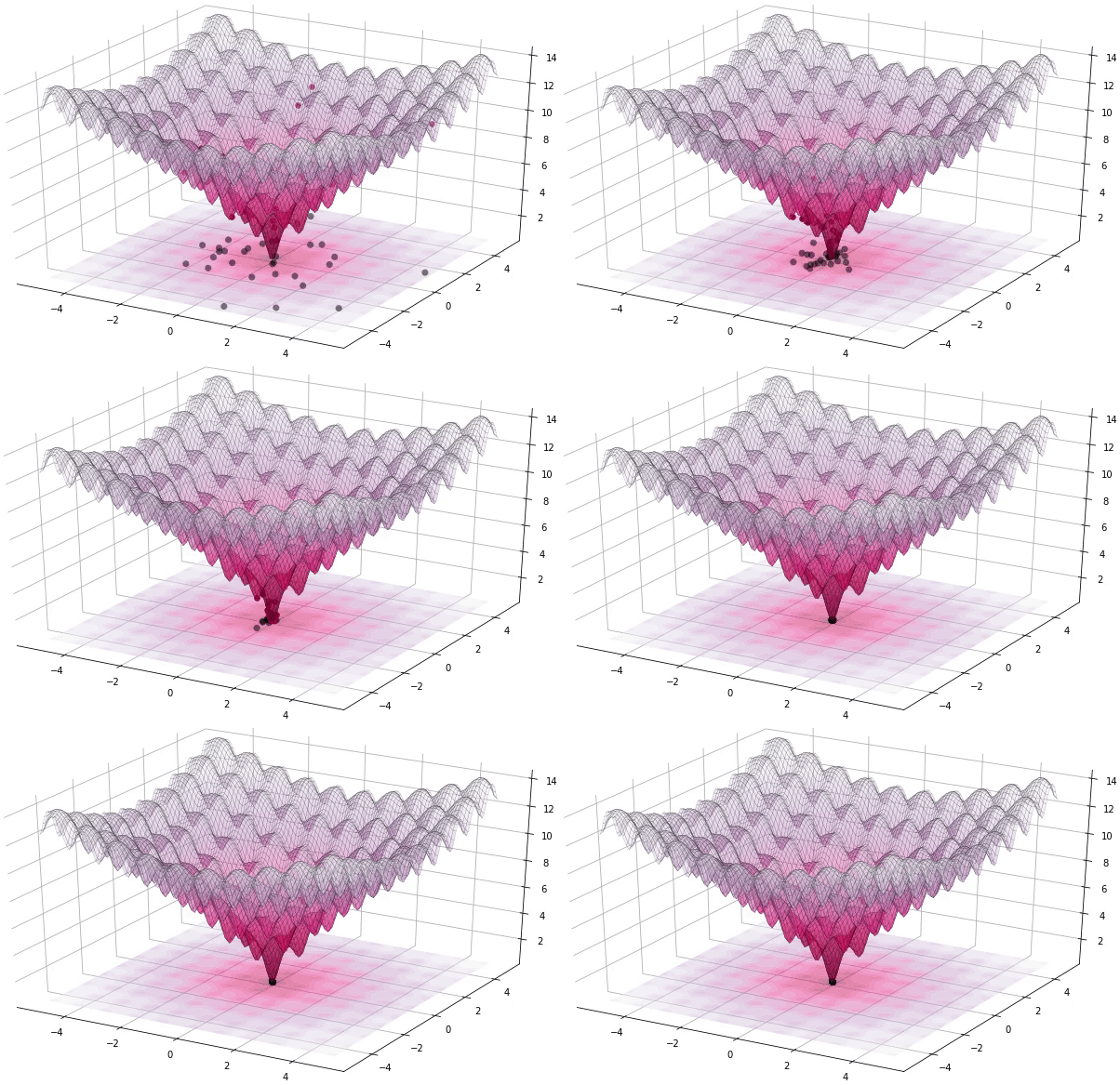
The optimization of black-box functions is very common in real world problems, where the function to be optimized is very complex (and may involve the use of simulators or external software for the computations). For these kind of problems, DE works pretty well, and that’s why it’s very popular for solving problems in many different fields, including Astronomy, Chemistry, Biology, and many more. For example, the European Space Agency (ESA) uses DE to design optimal trajectories in order to reach the orbit of a planet using as less fuel as possible. Sounds awesome right? Best of all, the algorithm is very simple to understand and to implement. In this tutorial, we will see how to implement it, how to use it to solve some problems and we will build intuition about how DE works.
Let’s start!
Before getting into more technical details, let’s get our hands dirty. One thing that fascinates me about DE is not only its power but its simplicity, since it can be implemented in just a few lines. Here is the code for the DE algorithm using the rand/1/bin schema (we will talk about what this means later). It only took me 27 lines of code using Python with Numpy:
This code is completely functional, you can paste it into a python terminal and start playing with it (you need numpy >= 1.7.0). Don’t worry if you don’t understand anything, we will see later what is the meaning of each line in this code. The good thing is that we can start playing with this right now without knowing how this works. The only two mandatory parameters that we need to provide are fobj and bounds:
-
fobj: \(f(x)\) function to optimize. Can be a function defined with a
defor a lambda expression. For example, suppose we want to minimize the function \(f(x)=\sum_i^n x_i^2/n\). Ifxis a numpy array, our fobj can be defined as:fobj = lambda x: sum(x**2)/len(x)If we define
xas a list, we should define our objective function in this way:def fobj(x): value = 0 for i in range(len(x)): value += x[i]**2 return value / len(x) -
bounds: a list with the lower and upper bound for each parameter of the function. For example: \(bounds_x=\) [(-5, 5), (-5, 5), (-5, 5), (-5, 5)] means that each variable \(x_i, i \in [1, 4]\) is bound to the interval [-5, 5].
For example, let’s find the value of x that minimizes the function \(f(x) = x^2\), looking for values of \(x\) between -100 and 100:
>>> it = list(de(lambda x: x**2, bounds=[(-100, 100)]))
>>> print(it[-1])

(array([ 0.]), array([ 0.]))
The first value returned (array([ 0.]) represents the best value for x (in this case is just a single number since the function is 1-D), and the value of f(x) for that x is returned in the second array (array([ 0.]).
Note: for convenience, I defined the
defunction as a generator function that yields the best solution \(x\) and its corresponding value of \(f(x)\) at each iteration. In order to obtain the last solution, we only need to consume the iterator, or convert it to a list and obtain the last value withlist(de(...))[-1]
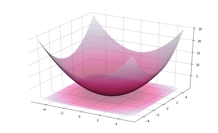
Yeah I know, this is too easy. Now, let’s try the same example in a multi-dimensional setting, with the function now defined as \(f(x) = \sum_{i}^n x_i^2 / n\), for n=32 dimensions. This is how it looks like in 2D:
# https://github.com/pablormier/yabox
# pip install yabox
>>> from yabox.problems import problem
>>> problem(lambda x: sum(x**2)/len(x), bounds=[(-5, 5)] * 2).plot3d()
>>> result = list(de(lambda x: x**2 / len(x), bounds=[(-100, 100)] * 32))
>>> print(result[-1])

(array([ 1.43231366,  4.83555112,  0.29051824,  2.94836318,  2.02918578,
       -2.60703144,  0.76783095, -1.66057484,  0.42346029, -1.36945634,
       -0.01227915, -3.38498397, -1.76757209,  3.16294878,  5.96335235,
        3.51911452,  1.24422323,  2.9985505 , -0.13640705,  0.47221648,
        0.42467349,  0.26045357,  1.20885682, -1.6256121 ,  2.21449962,
       -0.23379811,  2.20160374, -1.1396289 , -0.72875512, -3.46034836,
       -5.84519163,  2.66791339]), 6.3464570348900136)
This time the best value for f(x) was 6.346, we didn’t obtained the optimal solution \(f(0, \dots, 0) = 0\). Why? DE doesn’t guarantee to obtain the global minimum of a function. What it does is to approach the global minimum in successive steps, as shown in Fig. 1. So in general, the more complex the function, the more iterations are needed. This can raise a new question: how does the dimensionality of a function affects the convergence of the algorithm? In general terms, the difficulty of finding the optimal solution increases exponentially with the number of dimensions (parameters). This effect is called “curse of dimensionality”. For example, suppose we want to find the minimum of a 2D function whose input values are binary. Since they are binary and there are only two possible values for each one, we would need to evaluate in the worst case \(2^2 = 4\) combinations of values: \(f(0,0)\), \(f(0,1)\), \(f(1,0)\) and \(f(1,1)\). But if we have 32 parameters, we would need to evaluate the function for a total of \(2^{32}\) = 4,294,967,296 possible combinations in the worst case (the size of the search space grows exponentially). This makes the problem much much more difficult, and any metaheuristic algorithm like DE would need many more iterations to find a good approximation.
Knowing this, let’s run again the algorithm but for 3,000 iterations instead of just 1,000:
>>> result = list(de(lambda x: x**2 / len(x), bounds=[(-100, 100)] * 32, its=3000))
>>> print(result[-1])

(array([ 0.00648831, -0.00093694, -0.00205017,  0.00136862, -0.00722833,
       -0.00138284,  0.00323691,  0.0040672 , -0.0060339 ,  0.00631543,
       -0.01132894,  0.00020696,  0.00020962, -0.00063984, -0.00877504,
       -0.00227608, -0.00101973,  0.00087068,  0.00243963,  0.01391991,
       -0.00894368,  0.00035751,  0.00151198,  0.00310393,  0.00219394,
        0.01290131, -0.00029911,  0.00343577, -0.00032941,  0.00021377,
       -0.01015071,  0.00389961]), 3.1645278699373536e-05)
Now we obtained a much better solution, with a value very close to 0. In this case we only needed a few thousand iterations to obtain a good approximation, but with complex functions we would need much more iterations, and yet the algorithm could get trapped in a local minimum. We can plot the convergence of the algorithm very easily (now is when the implementation using a generator function comes in handy):
>>> import matplotlib.pyplot as plt
>>> x, f = zip(*result)
>>> plt.plot(f)
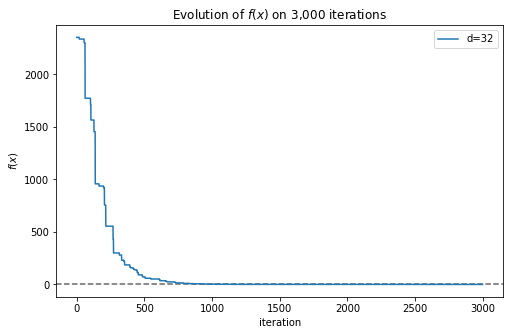
Fig. 3 shows how the best solution found by the algorithm approximates more and more to the global minimum as more iterations are executed. Now we can represent in a single plot how the complexity of the function affects the number of iterations needed to obtain a good approximation:
for d in [8, 16, 32, 64]:
    it = list(de(lambda x: sum(x**2)/d, [(-100, 100)] * d, its=3000))
    x, f = zip(*it)
    plt.plot(f, label='d={}'.format(d))
plt.legend()
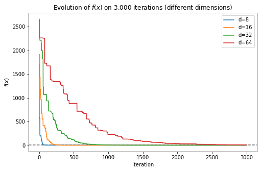
The plot makes it clear that when the number of dimensions grows, the number of iterations required by the algorithm to find a good solution grows as well.
How it works?
Now it’s time to talk about how these 27 lines of code work. Differential Evolution, as the name suggest, is a type of evolutionary algorithm. An evolutionary algorithm is an algorithm that uses mechanisms inspired by the theory of evolution, where the fittest individuals of a population (the ones that have the traits that allow them to survive longer) are the ones that produce more offspring, which in turn inherit the good traits of the parents. This makes the new generation more likely to survive in the future as well, and so the population improves over time, generation after generation. This is possible thanks to different mechanisms present in nature, such as mutation, recombination and selection, among others. Evolutionary algorithms apply some of these principles to evolve a solution to a problem.
In this way, in Differential Evolution, solutions are represented as populations of individuals (or vectors), where each individual is represented by a set of real numbers. These real numbers are the values of the parameters of the function that we want to minimize, and this function measures how good an individual is. The main steps of the algorithm are: initialization of the population, mutation, recombination, replacement and evaluation. Let’s see how these operations are applied working through a simple example of minimizing the function \(f(\mathbf{x})=\sum x_i^2/n\) for \(n=4\), so \(\mathbf{x}=\{x_1, x_2, x_3, x_4\}\), and \(-5 \leq x_i \leq 5\).
Components
- fobj:
fobj = lambda x: sum(x**2)/len(x) - bounds:
bounds = [(-5, 5)] * 4
Initialization
The first step in every evolutionary algorithm is the creation of a population with popsize individuals. An individual is just an instantiation of the parameters of the function fobj. At the beginning, the algorithm initializes the individuals by generating random values for each parameter within the given bounds. For convenience, I generate uniform random numbers between 0 and 1, and then I scale the parameters (denormalization) to obtain the corresponding values. This is done in lines 4-8 of the algorithm.
# Population of 10 individuals, 4 params each (popsize = 10, dimensions = 4)
>>> pop = np.random.rand(popsize, dimensions)
>>> pop

#        x[0]   x[1]   x[2]   x[3]
array([[ 0.09,  0.01,  0.4 ,  0.21],
       [ 0.04,  0.87,  0.52,  0.  ],
       [ 0.96,  0.78,  0.65,  0.17],
       [ 0.22,  0.83,  0.23,  0.84],
       [ 0.8 ,  0.43,  0.06,  0.44],
       [ 0.95,  0.99,  0.93,  0.39],
       [ 0.64,  0.97,  0.82,  0.06],
       [ 0.41,  0.03,  0.89,  0.24],
       [ 0.88,  0.29,  0.15,  0.09],
       [ 0.13,  0.19,  0.17,  0.19]])
This generates our initial population of 10 random vectors. Each component x[i] is normalized between [0, 1]. We will use the bounds to denormalize each component only for evaluating them with fobj.
Evaluation
The next step is to apply a linear transformation to convert each component from [0, 1] to [min, max]. This is only required to evaluate each vector with the function fobj:
>>> pop_denorm = min_b + pop * diff
>>> pop_denorm

array([[-4.06, -4.89, -1.  , -2.87],
       [-4.57,  3.69,  0.19, -4.95],
       [ 4.58,  2.78,  1.51, -3.31],
       [-2.83,  3.27, -2.72,  3.43],
       [ 3.  , -0.68, -4.43, -0.57],
       [ 4.47,  4.92,  4.27, -1.05],
       [ 1.36,  4.74,  3.19, -4.37],
       [-0.89, -4.67,  3.85, -2.61],
       [ 3.76, -2.14, -3.53, -4.06],
       [-3.67, -3.14, -3.34, -3.06]])
At this point we have our initial population of 10 vectors, and now we can evaluate them using our fobj. Although these vectors are random points of the function space, some of them are better than others (have a lower \(f(x)\)). Let’s evaluate them:
>>> for ind in pop_denorm:
>>>    print(ind, fobj(ind))

[-4.06 -4.89 -1.   -2.87] 12.3984504837
[-4.57  3.69  0.19 -4.95] 14.7767132816
[ 4.58  2.78  1.51 -3.31] 10.4889711137
[-2.83  3.27 -2.72  3.43] 9.44800715266
[ 3.   -0.68 -4.43 -0.57] 7.34888318457
[ 4.47  4.92  4.27 -1.05] 15.8691538075
[ 1.36  4.74  3.19 -4.37] 13.4024093959
[-0.89 -4.67  3.85 -2.61] 11.0571791104
[ 3.76 -2.14 -3.53 -4.06] 11.9129095178
[-3.67 -3.14 -3.34 -3.06] 10.9544056745
After evaluating these random vectors, we can see that the vector x=[ 3., -0.68, -4.43, -0.57] is the best of the population, with a \(f(x)=7.34\), so these values should be closer to the ones that we’re looking for. The evaluation of this initial population is done in L. 9 and stored in the variable fitness.
Mutation & Recombination
How can the algorithm find a good solution starting from this set of random values?. This is when the interesting part comes. Now, for each vector pop[j] in the population (from j=0 to 9), we select three other vectors that are not the current one, let’s call them a, b and c. So we start with the first vector pop[0] = [-4.06 -4.89 -1. -2.87] (called target vector), and in order to select a, b and c, what I do is first I generate a list with the indexes of the vectors in the population, excluding the current one (j=0) (L. 14):
>>> target = pop[j] # (j = 0)
>>> idxs = [idx for idx in range(popsize) if idx != j] # (j = 0)
>>> idxs

[1, 2, 3, 4, 5, 6, 7, 8, 9]
And then I randomly choose 3 indexes without replacement (L. 14-15):
>>> selected = np.random.choice(idxs, 3, replace=False)
>>> selected

array([1, 4, 7])
Here are our candidates (taken from the normalized population):
>>> pop[selected]

array([[ 0.04,  0.87,  0.52,  0.  ],  # a
       [ 0.8 ,  0.43,  0.06,  0.44],  # b
       [ 0.41,  0.03,  0.89,  0.24]]) # c

>>> a, b, c = pop[selected]
Now, we create a mutant vector by combining a, b and c. How? by computing the difference (now you know why it’s called differential evolution) between b and c and adding those differences to a after multiplying them by a constant called mutation factor (parameter mut). A larger mutation factor increases the search radius but may slowdown the convergence of the algorithm. Values for mut are usually chosen from the interval [0.5, 2.0]. For this example, we will use the default value of mut = 0.8:
# mut = 0.8
>>> mutant = a + mut * (b - c)

array([ 0.35,  1.19, -0.14,  0.17])
Note that after this operation, we can end up with a vector that is not normalized (the second value is greater than 1 and the third one is smaller than 0). The next step is to fix those situations. There are two common methods: by generating a new random value in the interval [0, 1], or by clipping the number to the interval, so values greater than 1 become 1, and the values smaller than 0 become 0. I chose the second option just because it can be done in one line of code using numpy.clip:
>>> np.clip(mutant, 0, 1)

array([ 0.35,  1.  ,  0.  ,  0.17])
Now that we have our mutant vector, the next step to perform is called recombination. Recombination is about mixing the information of the mutant with the information of the current vector to create a trial vector. This is done by changing the numbers at some positions in the current vector with the ones in the mutant vector. For each position, we decide (with some probability defined by crossp) if that number will be replaced or not by the one in the mutant at the same position. To generate the crossover points, we just need to generate uniform random values between [0, 1] and check if the values are less than crossp. This method is called binomial crossover since the number of selected locations follows a binomial distribution.
>>> cross_points = np.random.rand(dimensions) < crossp
>>> cross_points

array([False,  True, False,  True], dtype=bool)
In this case we obtained two Trues at positions 1 and 3, which means that the values at positions 1 and 3 of the current vector will be taken from the mutant. This can be done in one line again using the numpy function where:
>>> trial = np.where(cross_points, mutant, pop[j]) # j = 0
>>> trial

array([ 0.09,  1.  ,  0.4 ,  0.17])
Replacement
After generating our new trial vector, we need to denormalize it and evaluate it to measure how good it is. If this mutant is better than the current vector (pop[0]) then we replace it with the new one.
>>> trial_denorm = min_b + trial * diff
>>> trial_denorm

array([-4.1,  5. , -1. , -3.3])
And now, we can evaluate this new vector with fobj:
>>> fobj(mutant_denorm)

13.425000000000001
In this case, the trial vector is worse than the target vector (13.425 > 12.398), so the target vector is preserved and the trial vector discarded. All these steps have to be repeated again for the remaining individuals (pop[j] for j=1 to j=9), which completes the first iteration of the algorithm. After this process, some of the original vectors of the population will be replaced by better ones, and after many iterations, the whole population will eventually converge towards the solution (it’s a kind of magic uh?).
Polynomial curve fitting example
Let’s see now the algorithm in action with another concrete example. Given a set of points (x, y), the goal of the curve fitting problem is to find the polynomial that better fits the given points by minimizing for example the sum of the distances between each point and the curve. For this purpose, we are going to generate our set of observations (x, y) using the function \(f(x)=cos(x)\), and adding a small amount of gaussian noise:
>>> x = np.linspace(0, 10, 500)
>>> y = np.cos(x) + np.random.normal(0, 0.2, 500)
>>> plt.scatter(x, y)
>>> plt.plot(x, np.cos(x), label='cos(x)')
>>> plt.legend()
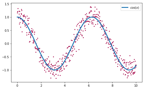
Our goal is to fit a curve (defined by a polynomial) to the set of points that we generated before. This curve should be close to the original \(f(x)=cos(x)\) used to generate the points.
We would need a polynomial with enough degrees to generate at least 4 curves. For this purpose, a polynomial of degree 5 should be enough (you can try with more/less degrees to see what happens):
\[f_{model}(\mathbf{w}, x) = w_0 + w_1 x + w_2 x^2 + w_3 x^3 + w_4 x^4 + w_5 x^5\]
This polynomial has 6 parameters \(\mathbf{w}=\{w_1, w_2, w_3, w_4, w_5, w_6\}\). Different values for those parameters generate different curves. Let’s implement it:
def fmodel(x, w):
    return w[0] + w[1]*x + w[2] * x**2 + w[3] * x**3 + w[4] * x**4 + w[5] * x**5
Using this expression, we can generate an infinite set of possible curves. For example:
>>> plt.plot(x, fmodel(x, [1.0, -0.01, 0.01, -0.1, 0.1, -0.01]))
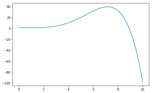
Among this infinite set of curves, we want the one that better approximates the original function \(f(x)=cos(x)\). For this purpose, we need a function that measures how good a polynomial is. We can use for example the Root Mean Square Error (RMSE) function:
def rmse(w):
    y_pred = fmodel(x, w)
    return np.sqrt(sum((y - y_pred)**2) / len(y))
Now we have a clear description of our problem: we need to find the parameters \(\mathbf{w}=\{w_1, w_2, w_3, w_4, w_5, w_6\}\) for our polynomial of degree 5 that minimizes the rmse function. Let’s evolve a population of 20 random polynomials for 2,000 iterations with DE:
>>> result = list(de(rmse, [(-5, 5)] * 6, its=2000))
>>> result

(array([ 0.99677643,  0.47572443, -1.39088333,  0.50950016, -0.06498931,
         0.00273167]), 0.214860061914732)
We obtained a solution with a rmse of ~0.215. We can plot this polynomial to see how good our approximation is:
>>> plt.scatter(x, y)
>>> plt.plot(x, np.cos(x), label='cos(x)')
>>> plt.plot(x, fmodel(x, [0.99677643, 0.47572443, -1.39088333,
>>>                        0.50950016, -0.06498931, 0.00273167]), label='result')
>>> plt.legend()
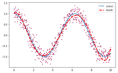
Not bad at all! Now let’s see in action how the algorithm evolve the population of random vectors until all of them converge towards the solution. It is very easy to create an animation with matplotlib, using a slight modification of our original DE implementation to yield the entire population after each iteration instead of just the best vector:
# Replace this line in DE (L. 29)
yield best, fitness[best_idx]
# With this line (and call the new version de2)
yield min_b + pop * diff, fitness, best_idx
import matplotlib.animation as animation
from IPython.display import HTML

result = list(de2(rmse, [(-5, 5)] * 6, its=2000))

fig, ax = plt.subplots()

def animate(i):
    ax.clear()
    ax.set_ylim([-2, 2])
    ax.scatter(x, y)
    pop, fit, idx = result[i]
    for ind in pop:
        data = fmodel(x, ind)
        ax.plot(x, data, alpha=0.3)
Now we only need to generate the animation:
>>> anim = animation.FuncAnimation(fig, animate, frames=2000, interval=20)
>>> HTML(anim.to_html5_video())
The animation shows how the different vectors in the population (each one corresponding to a different curve) converge towards the solution after a few iterations.
DE variations
The schema used in this version of the algorithm is called rand/1/bin because the vectors are randomly chosen (rand), we only used 1 vector difference and the crossover strategy used to mix the information of the trial and the target vectors was a binomial crossover. But there are other variants:
Mutation schemas
- Rand/1: \(x_{mut} = x_{r1} + F(x_{r2} - x_{r3})\)
- Rand/2: \(x_{mut} = x_{r1} + F(x_{r2} - x_{r3} + x_{r4} - x_{r5})\)
- Best/1: \(x_{mut} = x_{best} + F(x_{r2} - x_{r3})\)
- Best/2: \(x_{mut} = x_{best} + F(x_{r2} - x_{r3} + x_{r4} - x_{r5})\)
- Rand-to-best/1: \(x_{mut} = x_{r1} + F_1(x_{r2} - x_{r3}) + F_2(x_{best} - x_{r1})\)
- …
Crossover schemas
- Binomial (bin): crossover due to independent binomial experiments. Each component of the target vector has a probability p of being changed by the component of the the mutant vector.
- Exponential (exp): it’s a two-point crossover operator, where two locations of the vector are randomly chosen so that n consecutive numbers of the vector (between the two locations) are taken from the mutant vector.
Mutation/crossover schemas can be combined to generate different DE variants, such as rand/2/exp, best/1/exp, rand/2/bin and so on. There is no single strategy “to rule them all”. Some schemas work better on some problems and worse in others. The tricky part is choosing the best variant and the best parameters (mutation factor, crossover probability, population size) for the problem we are trying to solve.
Final words
Differential Evolution (DE) is a very simple but powerful algorithm for optimization of complex functions that works pretty well in those problems where other techniques (such as Gradient Descent) cannot be used. In this post, we’ve seen how to implement it in just 27 lines of Python with Numpy, and we’ve seen how the algorithm works step by step.
If you are looking for a Python library for black-box optimization that includes the Differential Evolution algorithm, here are some:
-
Yabox. Yet another black-box optimization library for Python 3+. This is a project I’ve started recently, and it’s the library I’ve used to generate the figures you’ve seen in this post. Yabox is a very lightweight library that depends only on Numpy.
-
Pygmo. A powerful library for numerical optimization, developed and mantained by the ESA. Pygmo is a scientific library providing a large number of optimization problems and algorithms under the same powerful parallelization abstraction built around the generalized island-model paradigm.
-
Platypus. Platypus is a framework for evolutionary computing in Python with a focus on multiobjective evolutionary algorithms (MOEAs). It differs from existing optimization libraries, including PyGMO, Inspyred, DEAP, and Scipy, by providing optimization algorithms and analysis tools for multiobjective optimization
-
Scipy. The well known scientific library for Python includes a fast implementation of the Differential Evolution algorithm. . n algorithm.